Note 5 Relational Database Design and Normalization
Author: Zhen Tong 120090694@link.cuhk.edu.cn Lecturer: Jan YOU
Before Everything
This note will mainly focus on what is a suitable schema.
A Good Design
Before learning the idea of a good design, let’s see what is bad first.
Update Anomaly
Take the example from the lecture:
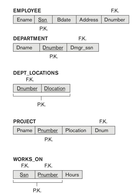
If we change to another design like this:
EMP_PROJ
| EmpSsn | Pnumber | Ename | Pname | No_hours |
We combine the Employee with the Project, which can be a bad design, because, now when we want to change the name of this project from "Billing" to "Customer Accounting" (presumably because the project's focus has changed), this update operation may have unintended consequences.
The anomaly suggests that making this change for "P1" might result in the name of the project being updated for all the employees who are working on the project "P1," even if they are still working on the original "Billing" project. This is an anomaly because the update operation is affecting more data than what was initially intended.
This problem is called Update Anomaly.
Insertion Anomaly
Still this schema, it can cause Insertion Anomaly
- Cannot naturally insert a project unless an employee is assigned to it
- Conversely, cannot insert an employee unless he/she is assigned to a project
This part of the statement suggests that you can't add information about an employee to the database unless that employee is already assigned to a project and vice versa. In other words, employee records depend on project assignments, and you can't add employees unless they are working on a project.
Redundancy
Besides insertion and update anomaly, redundancy is also a problem. Look at this table below:
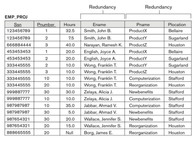
In the EMP_PROJ table, the Ename, Pname, and the Plocation are redundantly stored. I guess someone may come up with a question. “These data are not redundant, they are useful! You can visit them directly without using join, therefore it is time-saving!”
To answer this question, let’s do some math. Suppose you have employees and projects, and the redundancy data number is . As long as you increase one new entry in either employees or projects, you will need to consume or space to store the redundant data. However, in the original design, only space is used.
First Normal Form
After we know what is a bad design, let's introduce the main idea of normalization in this note.
In 1NF, a relational schema is organized in a specific way to ensure that data is stored and retrieved efficiently and without redundancy.
The key idea of the First Normal Form is the concept of an "atomic" domain, which means that the values in a column (attribute) of a relational table should be indivisible or considered as single, discrete units. In other words, each value in a column should be a simple, elementary piece of data, not a collection of related or grouped data.
For example, the university has courses like “csc3170”, “mat2050” the first letters are the subject, and the numbers are unique number in that subject. Then, this is not a atomic domain, because it can be further decomposed.
Also, let’s see how can we improve the example we have above EMP_PROJ
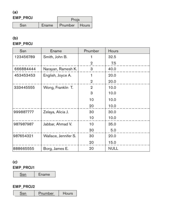
Do you still remember the update problem we have? Decomposition of EMP_PROJ into relations EMP_PROJ1 and EMP_PROJ2 by propagating the primary key. Then we can update either of them independently.
Functional Dependency and Decomposition
From the 2 example above, we know the first normalization always decompose larger design into smaller one. But does the decomposed structure always be a good design? What problems can it cause, and how can we detect them?
First, let’s define an important relationship among attribute, functional dependency
A functional dependency is denoted as , where X is the determinant attribute(s), and Y is the dependent attribute(s). This means that for every unique combination of values in X, there is a unique value of Y.
Here's an example to illustrate functional dependency:
Let's say we have a table called "Students" with the following attributes:
- Student_ID (unique identifier for each student)
- Student_Name (the name of the student)
- Student_Age (the age of the student)
- Student_Grade (the grade or class the student is in)
In this scenario, we can observe functional dependencies:
- Student_ID →Student_Name:
- Every unique Student_ID is associated with a unique Student_Name. For a given Student_ID, there is only one corresponding Student_Name.
- Student_ID → Student_Age:
- Similarly, each Student_ID is associated with a unique Student_Age. For a given Student_ID, there is only one corresponding Student_Age.
- Student_ID → Student_Grade:
- Again, there is a functional dependency. Each Student_ID is associated with a unique Student_Grade.
Lossless Decomposition
Then, let’s come back to the question: “does the decomposed structure always be a good design? “ Well, the answer is no. only the lossless decomposition is good.
For example
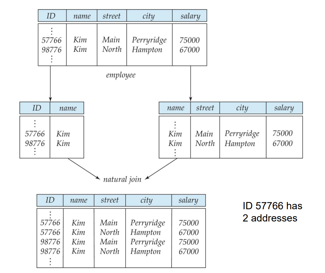
If we decompose the employee schema into two to store. When we need to use the merge data, we join them, then if two people have identical names, the join result will be in a number of , however, the right answer is 2, because there is only 2 person.
Formally, the decomposition of a relation shema is , and if we decompose it into , and join it back. Any entry in the , then decomposed into and should join to only as . i.e. . Conversely a decomposition is lossy if
Closure
Closure is a set conception, and I want to spare more time and effort to define everything clear.
A "closure" refers to the set of all functional dependencies that can be logically implied or derived from a given set of functional dependencies. The closure helps us determine all the relationships between attributes (columns) in a database based on the initial set of dependencies.
Here's an explanation of the concept:
- Set of Functional Dependencies (F): This is the initial set of functional dependencies that you have in a database. Each functional dependency in this set consists of an implication between two sets of attributes. For example, "A -> B" means that attribute A determines attribute B.
- Closure of F (F+): The closure of F, denoted as F+, is the set of all functional dependencies that can be logically derived from the initial set F. In other words, F+ contains all the dependencies that are implied by the transitive and reflexive properties of functional dependencies.
- Transitive Property: If you have functional dependencies A -> B and B -> C, you can infer the dependency A -> C. This means that if A determines B, and B determines C, then A determines C.
- Reflexive Property: Every attribute determines itself, so if you have a dependency A, you can consider it as A -> A.
By applying these properties, you can determine all the implied functional dependencies within the database. The closure F+ ensures that you have a complete and consistent understanding of how attributes depend on one another in your database schema.
Here's an example to illustrate the concept:
Suppose you have the following set of functional dependencies:
- A → B
- B v C
From these dependencies, you can derive the following implied dependencies:
- A → C (using the transitive property)
So, in this case, the closure F+ includes:
- A → B
- B →C
- A → C
The closure F+ provides a comprehensive understanding of the relationships between attributes based on the initial set of functional dependencies.
Keys and Functional Dependencies
Hope you still remember the conception of superkey, candidate key, primary key, and secondary key. Here is a recap:
- K is a superkey for relation schema R if and only if K → R
- K is a candidate key for R if and only if
- K→R, and
- for no
- One of the candidate keys is designated to be the primary key, and the others can be called secondary keys
- All data fields other than the pk can be called secondary key
Here introduce some new concepts:
- A prime attribute is a member of some candidate's key
- If there is only one candidate key – the primary key – then a prime attribute is an attribute that is a member of the primary key
- A nonprime attribute is not a prime attribute — that is, it is
not a member of any candidate key
- If there is only one candidate key – the primary key – then a nonprime attribute is an attribute that is not a member of the primary key
Trivial Functional Dependencies
- When , and , then it is trivial
It is called trivial because it doesn’t tell you any extra information, because it is self-contained in the original FD.
for example:
-
-
Lossless Decomposition and Functional Dependency Property
From above, we know that is a lossless decomposition. This can be equal to this property.
A decomposition of R into and is lossless decomposition if at least one of the following dependencies is in the closure of functional dependency of and
-
-
Let me further explain this condition. First is the part we can according to when do the join operation. I would like to metaphor this part as the zipper-zigzag part of the operation of two tables

Either can we find the unique right part on the right hand side, or should we able to find the unique left part of according to the zigzag intersection. Image if we can find more than one counterpart, what will the joined table like? The zipzag will be much longer isn’t it. which means the cloth will broke with this wrong zipzag.
Here is an example:
Because
and
This is a lossless decomposition.
Second Normal Form
Full functional dependency: an FD Y → Z where removal of any attribute from Y means the FD does not hold anymore.
A relation schema R is in second normal form (2NF) if it is in first normal form, and every nonprime attribute A in R is fully functionally dependent on the primary key (assuming it is the only candidate key).
The thing we improve from partial FD 1NF design to fully FD 2NF design is doing decomposition again. We should iteratively check the secondary attributes and separate the partial FD, and change them into fully FD.
Eliminating Partial Functional Dependencies
2NF helps reduce data redundancy by ensuring that non-prime attributes depend on the entire primary key. This means that for a relation to be in 2NF, non-prime attributes are functionally dependent on the entire primary key, and there are no partial dependencies. By adhering to 2NF, you store data efficiently, without duplication.
Third Normal Form
Transitive functional dependency: an FD X→Z that can be derived from two FDs X → Y and Y → Z, where Y is a nonprime attribute
3NF:
A relation schema R is in third normal form (3NF) if it is in 2NF and no nonprime attribute A in R is transitively dependent on the primary key (assuming it is the only candidate key)
Let’s further look at this two example.
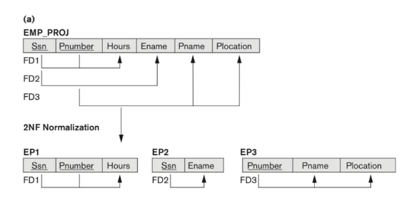
A tip in doing 2NF normalization task is look secondary attribute one by one to see if it is partial FD. The Hours is dependent on the Ssn and Pnumber. The Eame is only depend on the Ssn, and Pname, and Plocation is depend on the Pnumber. Therefore there are 3 kinds of secondary keys. Because there is no transitive functional dependency, so we stop at the 2NF.
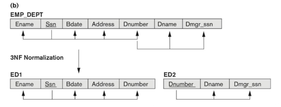
A tip in doing 3NF normalization task is look the dependency among secondary attributes. In the example of (b), we do the same thing, check the secondary attribute one-by-one, and we can find out the EMP_DEPT is already a 2NF. Because the Dnumber is not a pk in EMP_DEPT , and Dname, and Dmgr_ssn depend on it, we decomposite it into 3NF.
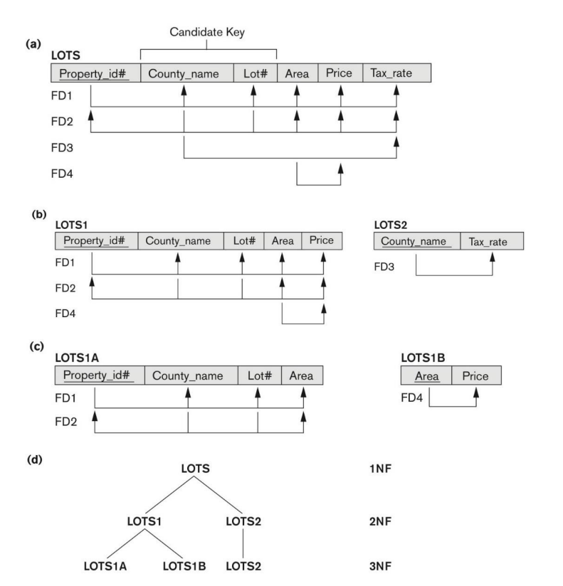
In this example, we first check partial FD, and find the County_name →Tax_rate is partial FD. Therefore do 2NF. Then we find out the Area → Price is a transitive FD. Continue do 3NF
General Normal Form
All the definitions of 1NF, 2NF, and 3NF are based on the primary key only. Then, what if there multiple candidate keys? The following statements are broadening the definition into more general world.
- prime attribute: any attribute that is a subset of a candidate key is a prime attribute.
- All other attributes are called non-prime attributes
A relation schema R is in second normal form (2NF) if it is in 1NF, and
every nonprime attribute A in R is fully functionally dependent on every
candidate key of R. You can refer to the situation of LOTS above.
To be more specific, consider another example:
- A is pk of R
- (B, C) is a candidate of R
- D depends on A, and B, i.e. (A, B)→D
Then, does this structure violate 2NF? No, it doesn’t although the candidate B, C is not fully depended by D explicitly, A→D itself is enough.
Boyce-Codd Normal Form(BCNF)
Before introduction of the BCNF, let’s first recap what is a superkey:
- Superkey of relation schema R - a set of attributes S of R that contains a candidate key of R
Then, the BCNF is defined based on the concept of Superkey:
- A relation schema R is in BCNF with respect to a set F of functional dependencies if for all functional dependencies in F+ of the form: where and , at least one of the following statement holds:
- is trivial
- is a superkey for
If we call the left hand side of an FD a determinant, like attributes, BCNF roughly says that every determinant is a superkey
For example:
in_dep
| ID | name | salary | dept_name | building | budget |
If there is one FD: dept_name → building, budget
This in_dep is not a BCNF, because dept_name itself is not a superkey, the superkey is ID, dept_name. Therefore to BCDF this in_dep, we need to decomposite into instructor and department:
instructor
| ID | name | salary | dept_name |
department
| dept_name | building | budget |
Decomposing a Schema into BCNF
With the above example, we can now translate the things we did into math language. Let R be a schema R that is not in BCNF. Let be the FD that causes a violation of BCNF, i.e. is not a superkey of R. To make the decomposited schema be BCNF, and maintain the functional dependency, we need to clean the . Here is again a metaphor, the violation of BCNF is like a cancer tumour on the body of the original schema. And the only way to fix is to cut the bad part, and remain the good part .
Therefore, the is decomposed into:
-
-
However, although we tried our best to maintain the dependency preserving, i.e. remain the original functional dependency closure, we still cannot guarantee the BCNF decomposition is perfectly dependency preserving.
Third Normal Form Revisited
2NF is 1NF, 3NF is 2NF, then, does BCNF a subset of 3NF? The 3NF is related to the Transitive functional dependency. The BCNF is related to superkey, then let’s see what is the definition of 3NF:
- A relation R is in 3NF if for all in , it is not a transitive functional dependency, which means at least one of the following holds:
- is trivial because a trivial dependency is not a transitive functional dependency.
- is a superkey for , because the determinant in transitive functional dependency is a non-primary attribute. If is a superkey, then, it cannot be partial FD, and cannot be a non-primary attribute.
- Each attribute A Each attribute A in is contained in a candidate key for R. For example, and are all candidate key, but exclusive. (NOTE: the third condition does not say that a single candidate key must contain all the attributes in ; each attribute A in may be contained in a different candidate key)
Therefore, if a relation is in BCNF it is in 3NF (since in BCNF one of the first two conditions above must hold). Third condition is a minimal relaxation of BCNF to ensure dependency preservation
However, a relation that is in 3NF but not in BCNF requires that for any nontrivial , is not a superkey but is a prime attribute
For example, schema dept_advisor
| s_ID | i_ID | dept_name |
The two candidate keys are {s_ID, dept_name}, {s_ID, i_ID }
- i_ID → dept_name
- s_ID, dept_name → i_ID
dept_advisor is not BCNF because i_ID is not a superkey
However, it is a 3NF,
i_ID → dept_name and i_ID is NOT a superkey, but
- { dept_name} – {i_ID } = {dept_name } and
- dept_name is contained in a candidate key
Pros and Cons in 3NF
It is always possible to obtain a 3NF design without sacrificing losslessness or dependency preservation
By definition of 3NF, this is 3NF
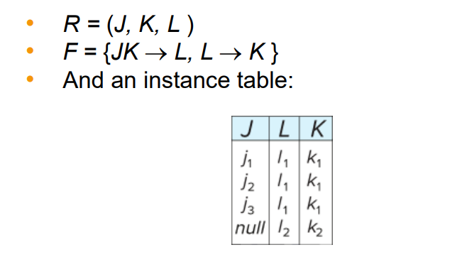
However, repetition of information (the association between L and K is repeated several times) Also, it needs to use null values (e.g., to represent the relationship where there is no corresponding value for J
Pros and Cons in BCNF
There are no non-trivial functional dependencies and therefore the relation is in BCNF. Insertion anomalies – i.e., if we add a phone 981-992-3443 to 99999, we need to add two tuples
(99999, David, 981-992-3443) (99999, William, 981-992-3443)